

Network-feasible allocation
TestingAllocations must remain within the physical limits of the electricity network.
Structured evidence
Claims, experimental inputs, simulations and published outputs used to evaluate this candidate electricity-market design.
Scientific claims
5 claims
Allocations must remain within the physical limits of the electricity network.
The mechanism must recognise that electricity and network capacity have different values at different locations.
When flexible capacity is insufficient, allocation should remain fair over time rather than being determined solely by willingness to pay.
Tested by
Persistent scarcity, network constraints, availability and substitutability should be reflected in long-run remuneration so that investment signals align with physical system value.
Tested by
Requests can be processed sequentially without requiring synchronised central scheduling of every participating device.
Tested by
Published evaluations
Experiment
A controlled network-constrained electricity-system benchmark used across the evidence programme. The scenario exposes persistent scarcity, transmission constraints, heterogeneous generation availability and differences in resource substitutability.
A valid market mechanism should respect the same underlying physical network constraints and scarcity conditions while producing feasible allocations and interpretable economic signals.
Run candidate mechanisms against an identical network, generation fleet, demand profile and temporal resolution, then translate outputs into a common canonical result schema.
The sections below present the experimental inputs, physical outcomes, economic comparison and generator-level fairness results. Individual simulation runs are retained in the evidence database for auditability but are not shown as part of the public narrative.
Investment signal theory
Shapley theory does not itself decide what "system value" means. That is defined by the characteristic function. In this experiment, the characteristic function is deliberately physical: it asks how much electrical demand can actually be served by a coalition of generators, given their availability, the location of demand and the capacity of the network.
Characteristic function
For a given half-hour t and coalition S, every generator outside the coalition is made unavailable. The optimisation then maximises physically served demand using only the generators in the coalition while respecting the network.
Generator constraint
0 ≤ pg,t ≤ p̄g,t, if g ∈ S
pg,t = 0, if g ∉ S
Served-demand constraint
0 ≤ sd,t ≤ Dd,t
Network constraint
−F̄ℓ ≤ Fℓ,t ≤ F̄ℓ
Nodal balance
generation + imports = served demand + exports
From coalition value to generator value
The Shapley value then asks how much generator g contributes on average when it is added to every possible coalition of the other generators. A generator therefore receives value for being useful when the system needs it, at a useful location, and when its contribution cannot easily be replaced by another resource.
Across the experimental horizon:
Worked example
This toy example shows why Shapley value is not simply installed capacity. The network changes how useful otherwise similar resources are to the system.
Node A
Demand: 50 MW
G1
Available capacity: 60 MW
Node B
Demand: 50 MW
G2
40 MW
G3
40 MW
| Coalition | v(S) | Why? |
|---|---|---|
| ∅ | 0 MW | No available generation, so no demand can be served. |
| {G1} | 60 MW | G1 can serve the 50 MW at Node A and export a further 10 MW across the line. |
| {G2} | 40 MW | G2 serves 40 MW of the 50 MW demand at Node B. |
| {G3} | 40 MW | G3 is symmetric with G2 in this toy system. |
| {G1, G2} | 100 MW | Together they can serve all 100 MW of system demand. |
| {G1, G3} | 100 MW | Together they can also serve all 100 MW of system demand. |
| {G2, G3} | 70 MW | They have 80 MW available at Node B, but Node B needs only 50 MW and the line can export only 20 MW. |
| {G1, G2, G3} | 100 MW | The grand coalition can serve all system demand. |
The key coalition
G2 and G3 together have 80 MW available, but their coalition is worth only 70 MW. Node B needs 50 MW and the line can export only 20 MW. An extra 10 MW behind the constraint cannot increase served demand, so it has no marginal system value in this state.
| Generator | Capacity | Capacity share | Shapley value | System-value share | Interpretation |
|---|---|---|---|---|---|
| G1 | 60 MW | 42.9% | 50 MW | 50% | Less substitutable because it is located on the opposite side of the constrained line. |
| G2 | 40 MW | 28.6% | 25 MW | 25% | Partly substitutable with G3 behind the same network constraint. |
| G3 | 40 MW | 28.6% | 25 MW | 25% | Symmetric with G2 and therefore receives the same Shapley value. |
What Shapley is rewarding
Availability: could the generator actually provide energy in the interval?
Timing: was its output available when demand was difficult to serve?
Location: could its output physically reach demand through the network?
Substitutability: could another generator have provided the same system service?
What Shapley is not doing
It does not assign technology-specific de-rating factors.
It does not assume that installed MW and useful MW are equivalent.
It does not derive generator value from the prevailing market price or scarcity rent.
The allocation follows from marginal contributions to the chosen physical characteristic function.
The fairness claim is conditional on the characteristic function
Shapley provides an axiomatically well-defined way to divide the value generated by a cooperative game. It does not remove the need to define the game itself. In this evidence framework, the governance choice is therefore concentrated in the characteristic function: what physical system outcome should count as value? Here, the answer is maximum servable demand subject to the actual network and availability constraints.
No published evidence is available for this experiment yet.
Experiment
Tests whether long-run generator remuneration can be allocated according to each resource's contribution to physical system value using a network-aware Shapley characteristic function.
If demand, network constraints, resource availability or substitutability change, coalition values and generator Shapley shares should change coherently with the underlying physical system need.
Calculate network-aware coalition values at each interval, allocate generator system value using Shapley theory, compare cost-recovery and equal-pot remuneration against LMP, decompose generator contributions, reconcile consumer cost recovery, and run controlled physical sensitivity tests.
The sections below present the experimental inputs, physical outcomes, economic comparison and generator-level fairness results. Individual simulation runs are retained in the evidence database for auditability but are not shown as part of the public narrative.
Experimental inputs
Both market mechanisms are evaluated against the same physical experiment: the same network topology, generator fleet, demand profiles, simulation horizon and temporal resolution. This section documents those inputs before any market result is interpreted.
Nodes
12
Network links
12
Generators
21
Loads
8
Intervals
336
30-minute resolution
The comparison uses a fixed experiment horizon and identical half-hourly system states for both mechanisms.
Start
1 Jan 2024, 00:00
End
7 Jan 2024, 23:30
Represented time
168 hours
The experiment combines an explicit network model, generator technical and cost assumptions, and synthetic residential demand. These inputs are fixed across the FP-AMM and LMP runs so that differences in the results reflect the market mechanism rather than a change in the physical scenario.
Network
The network is represented explicitly as buses and capacity-constrained links. Generators and loads are attached to specific nodes, allowing congestion and location to influence feasible dispatch and settlement.
Source file: network_uk.json
Generation
Generator inputs include node, technology, maximum output where applicable, minimum output, ramping capability, reserve capability and energy-cost assumptions. Storage units additionally include energy capacity, charging and discharging limits, efficiency and state-of-charge parameters.
Source file: gens_static.csv
Demand
Residential demand is synthetic and generated from four stylised household products, P1 to P4. The products vary in monthly energy use, maximum power and EV charging behaviour, producing heterogeneous rather than purely aggregate demand.
Demand type: synthetic
Controlled comparison
FP-AMM and LMP are evaluated against the same network, generation fleet, demand profiles and simulation horizon. This isolates the market-design effect: differences in dispatch, prices, scarcity outcomes and generator remuneration arise from the mechanism rather than from different physical inputs.
Generators and loads are attached to explicit network nodes. Power transfers between nodes are limited by the capacities of the connecting lines, so location and congestion are physical properties of the experiment rather than assumptions added later to the settlement.
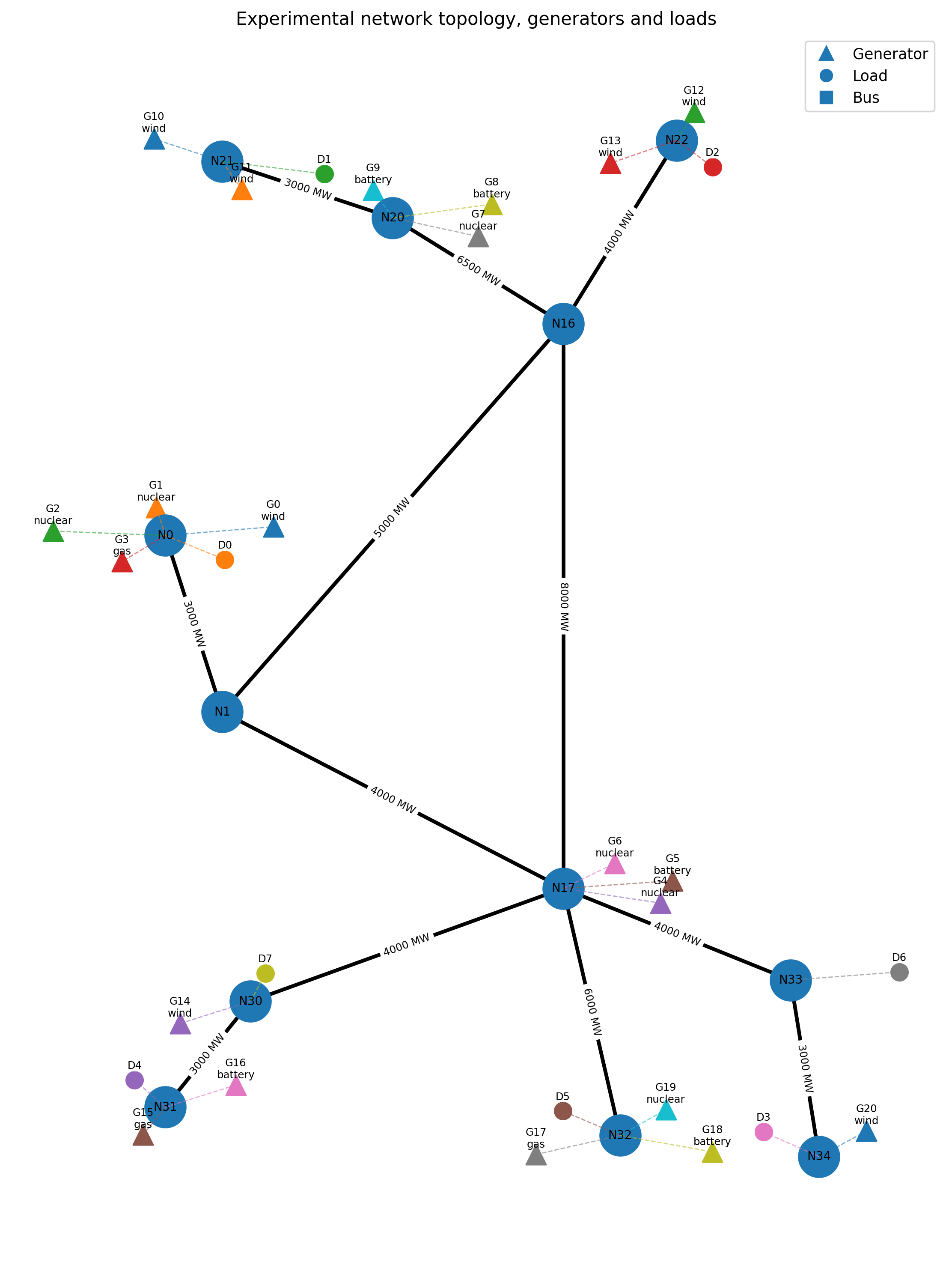
The topology figure shows buses, transmission links, line capacities, generator locations and load locations used by the experiment.
The same generator fleet is used under both market mechanisms. Technology and location determine the physical opportunities available to each generator, while the market design determines how those opportunities are valued and remunerated.
| Technology | Generators | Installed capacity | Non-fuel OPEX / yr | Annualised CAPEX |
|---|---|---|---|---|
| Battery | 5 | 4 GW | £70m | £186.67m |
| Gas | 3 | 35 GW | £700m | £1.98bn |
| Nuclear | 6 | 9.58 GW | £1.53bn | £1.68bn |
| Wind | 7 | 33.51 GW | £1.68bn | £3.18bn |
Installed capacity and fixed-cost assumptions come from the generator-cost input, while dispatch limits, marginal energy cost, reserve capability and storage characteristics come from the technical generator input.
| Generator | Node | Technology | Installed MW | Pmax | Pmin | Energy cost | Reserve | Storage | Non-fuel OPEX | Annualised CAPEX |
|---|---|---|---|---|---|---|---|---|---|---|
| G0 | N0 | Wind | 1.68 GW | — | 0 MW | £0/MWh | No | — | £83.77m | £159.15m |
| G1 | N0 | Nuclear | 2.4 GW | 2.4 GW | 1.2 GW | £12/MWh | No | — | £384m | £420m |
| G2 | N0 | Nuclear | 2.41 GW | 2.41 GW | 1.2 GW | £12/MWh | No | — | £384.8m | £420.88m |
| G3 | N0 | Gas | 12 GW | 12 GW | 2.4 GW | £90/MWh | Yes | — | £240m | £680m |
| G4 | N17 | Nuclear | 1.2 GW | 1.2 GW | 600 MW | £12/MWh | No | — | £192m | £210m |
| G5 | N17 | Battery | 500 MW | 500 MW | 0 MW | £70/MWh | Yes | 1 GWh | £8.75m | £23.33m |
| G6 | N17 | Nuclear | 1.17 GW | 1.17 GW | 585 MW | £12/MWh | No | — | £187.2m | £204.75m |
| G7 | N20 | Nuclear | 1.2 GW | 1.2 GW | 600 MW | £12/MWh | No | — | £192m | £210m |
| G8 | N20 | Battery | 1 GW | 1 GW | 0 MW | £70/MWh | Yes | 2 GWh | £17.5m | £46.67m |
| G9 | N20 | Battery | 1 GW | 1 GW | 0 MW | £70/MWh | Yes | 2 GWh | £17.5m | £46.67m |
| G10 | N21 | Wind | 6.7 GW | — | 0 MW | £0/MWh | No | — | £335.06m | £636.62m |
| G11 | N21 | Wind | 6.7 GW | — | 0 MW | £0/MWh | No | — | £335.06m | £636.62m |
| G12 | N22 | Wind | 3.35 GW | — | 0 MW | £0/MWh | No | — | £167.53m | £318.31m |
| G13 | N22 | Wind | 6.7 GW | — | 0 MW | £0/MWh | No | — | £335.06m | £636.62m |
| G14 | N30 | Wind | 3.35 GW | — | 0 MW | £0/MWh | No | — | £167.53m | £318.31m |
| G15 | N31 | Gas | 8 GW | 8 GW | 1.6 GW | £90/MWh | Yes | — | £160m | £453.33m |
| G16 | N31 | Battery | 1 GW | 1 GW | 0 MW | £70/MWh | Yes | 2 GWh | £17.5m | £46.67m |
| G17 | N32 | Gas | 15 GW | 15 GW | 3 GW | £90/MWh | Yes | — | £300m | £850m |
| G18 | N32 | Battery | 500 MW | 500 MW | 0 MW | £70/MWh | Yes | 1 GWh | £8.75m | £23.33m |
| G19 | N32 | Nuclear | 1.2 GW | 1.2 GW | 600 MW | £12/MWh | No | — | £192m | £210m |
| G20 | N34 | Wind | 5.03 GW | — | 0 MW | £0/MWh | No | — | £251.3m | £477.46m |
Residential demand is generated synthetically rather than treating all households as one homogeneous load. Four stylised household products are used to represent different combinations of monthly energy consumption, maximum power and EV charging behaviour.
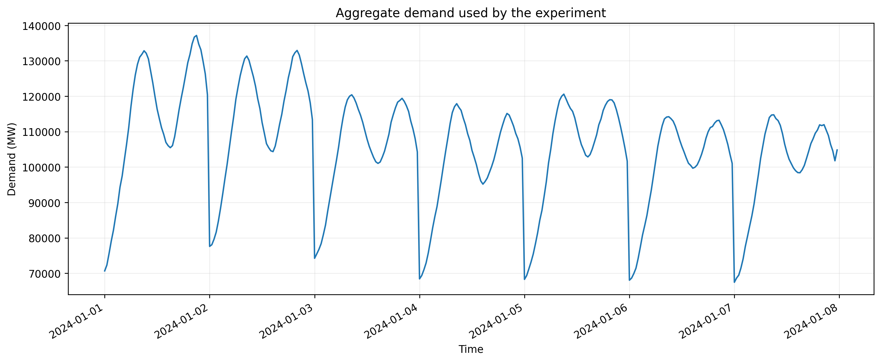
This is the aggregate half-hourly demand supplied directly to the market mechanism over the published experimental horizon. It is generated from the prepared demand inputs rather than reconstructed for presentation.
Average demand
105.71 GW
Peak demand
137.16 GW
Minimum demand
67.47 GW
Energy in horizon
17.76 TWh
P1 to P4 describe the heterogeneous household assumptions underneath the aggregate demand profile.
Product
Lower-power household with lower monthly energy consumption and no modelled EV charging.
Product
Higher-power, EV-capable household. EV charging is biased towards windier periods in the synthetic demand model.
Product
Lower-power household with higher monthly energy consumption and no modelled EV charging.
Product
Higher-power, EV-capable household with the highest target monthly energy consumption. EV charging is biased towards calmer periods in the synthetic demand model.
How the profiles are generated
Representative household profiles combine product-specific daily demand peaks, seasonal variation and reproducible stochastic variation. EV-capable products additionally receive synthetic charging sessions. The resulting product profiles are scaled towards their target monthly household energy consumption before being expanded to the modelled household population.
P2 and P4 include synthetic EV charging. P2 charging is biased towards windier periods; P4 charging is biased towards calmer periods.
Households
29m
Demand products
4
Profile type
Synthetic representative residential profiles
Calibration
Monthly energy
Reproducibility
Re-run the canonical scenario with the same network, generator, demand and market configuration inputs. The files published below document the prepared inputs and derived evidence associated with this run.
Run the canonical scenario through the pipeline using the same scenario.yaml and input files. The evidence outputs document the exact prepared inputs used by this run.
Command
python3 run.pyCanonical inputs
Network: network_uk.json
Generators: gens_static.csv
Generator costs: generator-costs.csv
Demand: demand
Resolution: 30 minutes
The machine-readable scenario and input summaries are published alongside the results so that the assumptions behind the experiment can be inspected directly.
Investment signal theory
Shapley theory does not itself decide what "system value" means. That is defined by the characteristic function. In this experiment, the characteristic function is deliberately physical: it asks how much electrical demand can actually be served by a coalition of generators, given their availability, the location of demand and the capacity of the network.
Characteristic function
For a given half-hour t and coalition S, every generator outside the coalition is made unavailable. The optimisation then maximises physically served demand using only the generators in the coalition while respecting the network.
Generator constraint
0 ≤ pg,t ≤ p̄g,t, if g ∈ S
pg,t = 0, if g ∉ S
Served-demand constraint
0 ≤ sd,t ≤ Dd,t
Network constraint
−F̄ℓ ≤ Fℓ,t ≤ F̄ℓ
Nodal balance
generation + imports = served demand + exports
From coalition value to generator value
The Shapley value then asks how much generator g contributes on average when it is added to every possible coalition of the other generators. A generator therefore receives value for being useful when the system needs it, at a useful location, and when its contribution cannot easily be replaced by another resource.
Across the experimental horizon:
Worked example
This toy example shows why Shapley value is not simply installed capacity. The network changes how useful otherwise similar resources are to the system.
Node A
Demand: 50 MW
G1
Available capacity: 60 MW
Node B
Demand: 50 MW
G2
40 MW
G3
40 MW
| Coalition | v(S) | Why? |
|---|---|---|
| ∅ | 0 MW | No available generation, so no demand can be served. |
| {G1} | 60 MW | G1 can serve the 50 MW at Node A and export a further 10 MW across the line. |
| {G2} | 40 MW | G2 serves 40 MW of the 50 MW demand at Node B. |
| {G3} | 40 MW | G3 is symmetric with G2 in this toy system. |
| {G1, G2} | 100 MW | Together they can serve all 100 MW of system demand. |
| {G1, G3} | 100 MW | Together they can also serve all 100 MW of system demand. |
| {G2, G3} | 70 MW | They have 80 MW available at Node B, but Node B needs only 50 MW and the line can export only 20 MW. |
| {G1, G2, G3} | 100 MW | The grand coalition can serve all system demand. |
The key coalition
G2 and G3 together have 80 MW available, but their coalition is worth only 70 MW. Node B needs 50 MW and the line can export only 20 MW. An extra 10 MW behind the constraint cannot increase served demand, so it has no marginal system value in this state.
| Generator | Capacity | Capacity share | Shapley value | System-value share | Interpretation |
|---|---|---|---|---|---|
| G1 | 60 MW | 42.9% | 50 MW | 50% | Less substitutable because it is located on the opposite side of the constrained line. |
| G2 | 40 MW | 28.6% | 25 MW | 25% | Partly substitutable with G3 behind the same network constraint. |
| G3 | 40 MW | 28.6% | 25 MW | 25% | Symmetric with G2 and therefore receives the same Shapley value. |
What Shapley is rewarding
Availability: could the generator actually provide energy in the interval?
Timing: was its output available when demand was difficult to serve?
Location: could its output physically reach demand through the network?
Substitutability: could another generator have provided the same system service?
What Shapley is not doing
It does not assign technology-specific de-rating factors.
It does not assume that installed MW and useful MW are equivalent.
It does not derive generator value from the prevailing market price or scarcity rent.
The allocation follows from marginal contributions to the chosen physical characteristic function.
The fairness claim is conditional on the characteristic function
Shapley provides an axiomatically well-defined way to divide the value generated by a cooperative game. It does not remove the need to define the game itself. In this evidence framework, the governance choice is therefore concentrated in the characteristic function: what physical system outcome should count as value? Here, the answer is maximum servable demand subject to the actual network and availability constraints.
Turning system value into remuneration
The Shapley calculation determines how system value is divided between generators. A separate question is how large the fixed-cost remuneration pot should be. The evidence therefore reports two cases: the proposed cost-recovery architecture and an equal-pot experimental comparison against LMP.
Generator fixed-cost requirement
Fuel and other marginal operating costs remain in the operational energy price. The separate investment layer is intended to recover non-fuel operating expenditure and annualised capital expenditure.
Proposed architecture
This case asks how much non-energy remuneration the modelled fleet actually requires, then allocates that requirement according to measured Shapley system value.
Operational market revenue
£342.3m
Shapley fixed-cost allocation
£210.5m
Total remuneration
£552.8m
Economic interpretation
The size of the fixed-cost pot comes from the generators' modelled non-fuel OPEX and annualised CAPEX requirements. Shapley determines how that pot is distributed according to physical system contribution.
Controlled comparison
This is not the proposed revenue requirement. It forces aggregate FP-AMM remuneration to equal aggregate LMP remuneration so that the distribution of the same money can be compared directly.
Operational market revenue
£342.3m
Equalising Shapley pot
£1.87bn
FP-AMM equal-pot total
£2.21bn
LMP comparison total
£2.21bn
Experimental interpretation
Because the aggregate remuneration is held constant, every gain by one generator is matched by a loss elsewhere. The experiment therefore isolates the allocation rule rather than the total amount of money recovered from the system.
1 · Determine requirement
Calculate each generator's non-fuel OPEX and annualised CAPEX requirement.
2 · Measure contribution
Calculate network-aware Shapley system value from the physical characteristic function.
3 · Allocate remuneration
Allocate the relevant pot according to the measured contribution rather than a technology-specific administrative factor.
Do not confuse the equal-pot result with the proposed FP-AMM revenue requirement
The equal-pot case exists only to make the distributional comparison with LMP clean. The proposed architecture is the cost-recovery case: marginal operating costs are recovered through the operational market, while non-fuel OPEX and annualised CAPEX are recovered separately through the Shapley investment signal.
Demand-side evidence
The consumer-side analysis applies the canonical IndividualTS_Base methodology. Costs are allocated half-hour by half-hour from the physical system state, then accumulated by P1-P4 and converted into a monthly-equivalent household charge.
Scarcity by design
This experiment deliberately operates under persistent scarcity so the allocation mechanism is tested when not all requested demand can be served. Requested, served and unserved demand are therefore reported separately. The household-cost calculation is based on the service actually delivered during the experiment.
Households represented
29,000,000
Demand served
84.9%
Across P1-P4 over the scarcity experiment.
Lowest monthly equivalent
£17.40
Highest monthly equivalent
£75.22
Fuel is allocated according to each product's share of controllable served energy. Non-fuel generator costs are allocated each half-hour using the product's capacity-weighted controllable demand. P2 and P4 therefore carry a higher capacity weighting than P1 and P3.
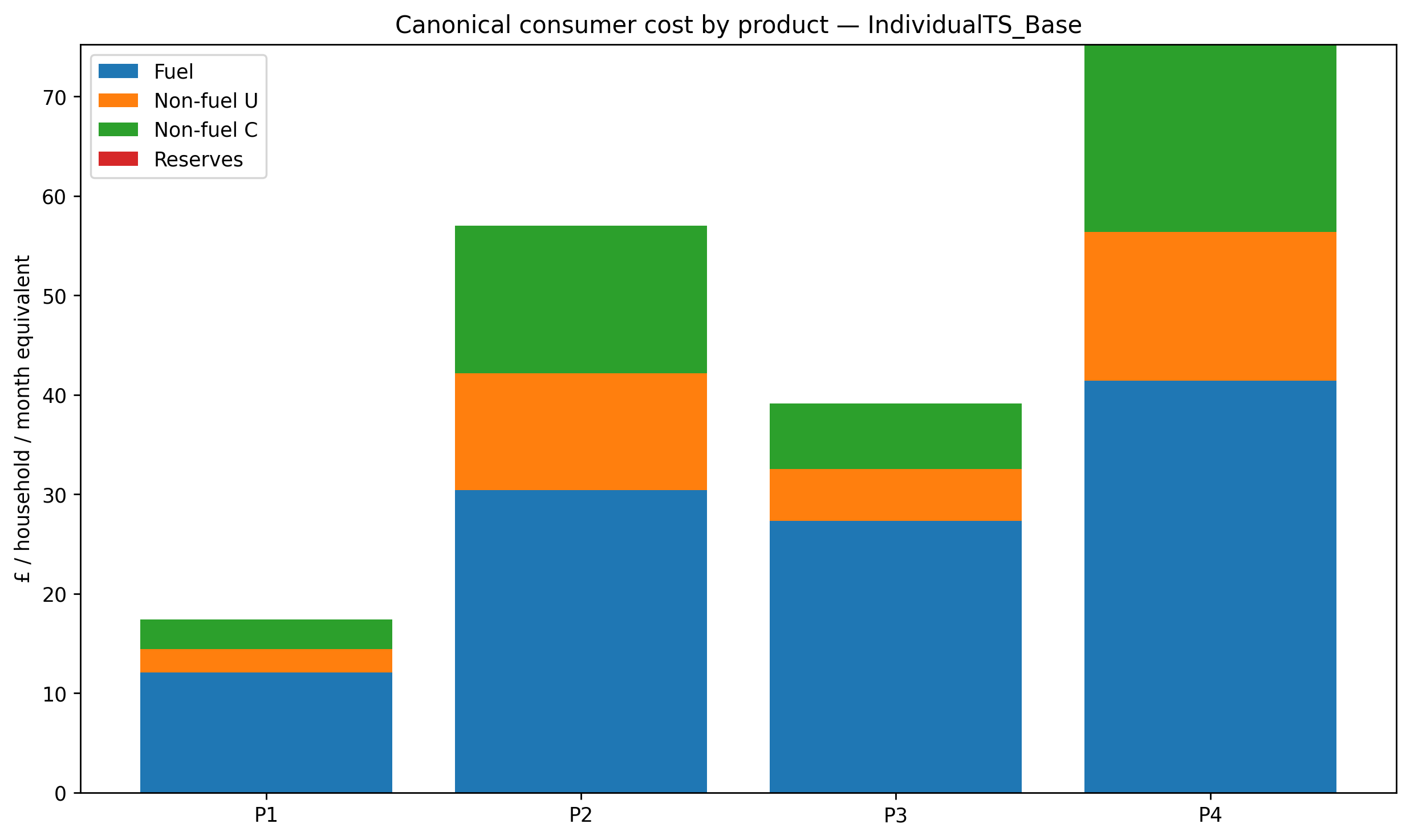
| Product | Requested | Served | Served share | Annualised kWh / HH | Fuel / month | Non-fuel U | Non-fuel C | Reserves | Total / month |
|---|---|---|---|---|---|---|---|---|---|
| P1 | 1.19 TWh | 1.01 TWh | 85% | 2,782 | £12.09 | £2.34 | £2.96 | £0.00 | £17.40 |
| P2 | 956.75 GWh | 814.84 GWh | 85.2% | 7,101 | £30.43 | £11.73 | £14.84 | £0.00 | £57.00 |
| P3 | 344.83 GWh | 291.88 GWh | 84.6% | 6,104 | £27.29 | £5.22 | £6.61 | £0.00 | £39.12 |
| P4 | 308.64 GWh | 259.51 GWh | 84.1% | 9,046 | £41.44 | £14.91 | £18.87 | £0.00 | £75.22 |
The physical demand allocation is retained alongside the financial result. U represents wind generation and C represents the controllable generation class used by the canonical consumer-cost methodology.
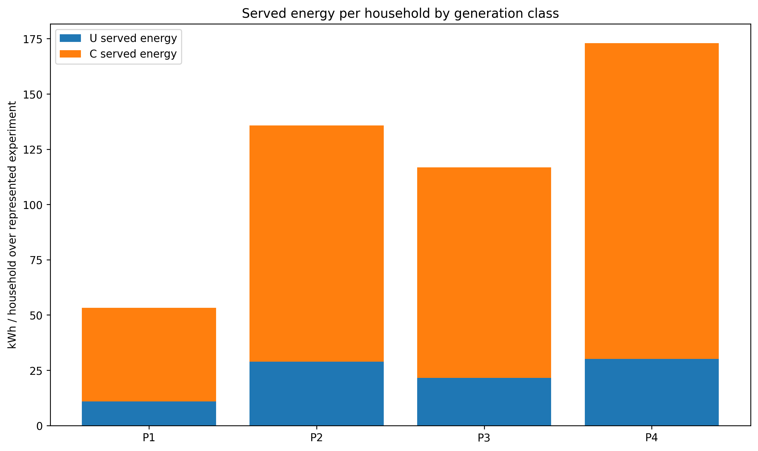
Why P2 can cost more than P3
The tariff is not purely volumetric. P2 and P4 have a higher capacity weight than P1 and P3, so a higher-power household can contribute more towards fixed system costs even when its total energy use is comparable with another product.
Exact accounting reconciliation
The published allocation reconciles exactly: fuel, non-fuel costs and the final product totals contain no unexplained residual.
View reconciliationMethodology
Canonical consumer-cost method. At each interval, fuel is allocated using controllable served-energy shares and BASE non-fuel generator-revenue pots are allocated using capacity-weighted controllable MW. Residential reserves are allocated uniformly per household.
The monthly values are annualised equivalents derived from 168 represented hours. They are not obtained by treating the seven-day experiment as a complete year.
Machine-readable methodologyCanonical results comparison
The latest published FP-AMM and LMP runs are compared using the same canonical result definitions. Values are automatically scaled for readability.
| Metric | FP-AMM | LMP | FP-AMM − LMP |
|---|---|---|---|
Served demand Total demand supplied during the experiment. | 6.32 TWh | 6.32 TWh | −0 MWh |
Unserved demand Demand that could not be supplied. | 1.16 TWh | 1.16 TWh | +0 MWh |
Unserved demand share Unserved demand as a percentage of total demand. | 15.6% | 15.6% | 0 pp |
Maximum price Highest settlement price observed during the run. | £90/MWh | £5,000/MWh | −£4,910/MWh |
Scarcity intervals Intervals in which physical scarcity was recorded. | 802 | 803 | −1 |
Scarcity energy Energy associated with intervals of physical scarcity. | 327.5 GWh | 309.3 GWh | +18.2 GWh |
Consumer payment Total payment attributed to served demand. | £342.34m | £6.7bn | −£6.36bn |
Generator revenue Total energy and reserve revenue paid to generators. | £552.84m | £2.21bn | −£1.66bn |
Production cost Total production cost derived from dispatch. | £341.84m | £342.01m | −£178.1k |
Generator net revenue Generator revenue less production cost. | £211.01m | £1.87bn | −£1.66bn |
FP-AMM run
thesis-network__amm__model-0.1.0__20260802T221657Z
LMP run
thesis-network__lmp__model-0.1.0__20260731T153839Z
Differences are reported as FP-AMM minus LMP. Interpretation should account for the shared scenario assumptions and the meaning of each settlement rule.
Distributional evidence
The physical experiment is held constant: the same network, demand, generation fleet and simulation horizon are used. The comparison then asks two different economic questions. The cost-recovery case measures the remuneration implied by the FP-AMM architecture itself. The equal-pot case holds total generator remuneration equal to LMP and examines how that same money is redistributed when system contribution is introduced explicitly through Shapley value.
These are not competing versions of the mechanism. They answer different questions. AMM1 asks what generators receive when the non-energy layer recovers modelled non-fuel OPEX and annualised CAPEX. AMM2 is a controlled fairness experiment in which the total remuneration pot is forced to equal the LMP total.
| Approach | Market settlement | Capacity / availability | Total remuneration |
|---|---|---|---|
| FP-AMM — cost recovery | £342.3m | £210.5m | £552.8m |
| FP-AMM — equal pot | £342.3m | £1.87bn | £2.21bn |
| LMP | £2.21bn | £0 | £2.21bn |
In the equal-pot experiment, FP-AMM and LMP distribute the same total remuneration: £2.21bn. The difference is therefore not the amount of money in the system, but who receives it and on what basis.
Once aggregate remuneration is fixed, every gain under FP-AMM is matched by a loss elsewhere. The resulting movement therefore measures redistribution rather than additional system cost.
Revenue redistributed
£1.7bn
Half of the absolute generator-level revenue movement, avoiding double-counting gains and matching losses.
Generators gaining
8
Generators receiving more under the FP-AMM equal-pot allocation than under LMP.
Generators losing
13
Generators receiving less under the FP-AMM equal-pot allocation than under LMP.
Shapley value is calculated independently from the market settlement and represents each generator's marginal contribution to the network-constrained system. The comparison below tests how closely each remuneration allocation follows that system-value signal.
| Measure | LMP | FP-AMM equal pot |
|---|---|---|
Pearson correlation Correlation between each generator's remuneration share and its Shapley system-value share. | 0.09 | 0.995 |
Mean absolute deviation Average absolute difference between remuneration share and Shapley system-value share. Lower is closer. | 6.54 pp | 1.89 pp |
Fairness here does not mean equal payment.
The design objective is to make remuneration more consistent with measured marginal system contribution. A generator that provides unusually high system value can therefore receive more than other generators without that being treated as a fairness failure. Conventional concentration statistics are useful diagnostics, but they answer a different question from alignment with system value.
In this published run, holding the total remuneration pot constant causes £1.7bn to change recipient. At the same time, the Pearson relationship between remuneration share and Shapley system value changes from 0.09 under LMP to 0.995 under FP-AMM, while mean absolute deviation falls from 6.54 pp to 1.89 pp.
Evidence run
thesis-network__amm__model-0.1.0__20260802T221657Z
The equal-pot comparison is a controlled distributional experiment. It should not be interpreted as the proposed FP-AMM cost-recovery requirement. The cost-recovery and equal-pot variants answer different questions and are reported separately.
System-value decomposition
The final Shapley share is the result of many marginal-contribution calculations across time and across alternative coalitions. The purpose of this decomposition is to make that result interpretable: was the generator available when scarcity mattered, could its output reach demand, and how easily could another resource replace it?
1 · Availability
How much capacity could the generator actually provide over the experiment?
2 · Timing
Was that availability present during the intervals when demand was difficult to serve?
3 · Location
Could the available output physically reach demand through the constrained network?
4 · Substitutes
How much extra demand did the generator serve after accounting for what the coalition could already do?
Contribution persistence in this scarcity experiment
Because this experiment deliberately maintains persistent scarcity, many generators make a positive marginal contribution in every interval. A contribution persistence of 100% is therefore not, by itself, the important distinction. The more informative signal is the magnitude of the generator's marginal contribution, together with how that contribution changes with availability, location and the presence of substitutes.
Gas · N32
Average availability
15,000 MW
Scarcity-weighted availability
15,000 MW
Contribution persistence
100%
Mean marginal contribution
13,630.01 MW
Investment-signal interpretation
This generator contributes more system value than a simple capacity-proportional allocation would imply. Its location, timing, availability or lack of effective substitutes increases its average marginal contribution.
Cost-recovery revenue
£25.42m
Equal-pot revenue
£775.59m
LMP revenue
£219.75m
Wind · N21
Average availability
1,342.7 MW
Scarcity-weighted availability
1,232.6 MW
Contribution persistence
100%
Mean marginal contribution
969.62 MW
Investment-signal interpretation
This generator contributes less system value than a simple capacity-proportional allocation would imply. Some of its installed or available capacity is comparatively substitutable or less able to increase served demand under the prevailing network state.
Cost-recovery revenue
£18.58m
Equal-pot revenue
£18.58m
LMP revenue
£412.41m
Capacity share is included as a simple reference point. A positive difference means that the generator's Shapley system-value share is greater than its share of installed capacity; a negative difference means the opposite.
| Generator | Node | Technology | Availability | Scarcity-weighted | Mean marginal | Max marginal | Contribution persistence | Capacity share | Shapley share | Δ share | Equal-pot revenue | LMP revenue |
|---|---|---|---|---|---|---|---|---|---|---|---|---|
| G17 | N32 | Gas | 15,000 MW | 15,000 MW | 13,630.01 MW | 14,807.83 MW | 100% | 18.3% | 32.6% | +14.3% | £775.59m | £219.75m |
| G15 | N31 | Gas | 8,000 MW | 8,000 MW | 7,269.34 MW | 7,897.51 MW | 100% | 9.7% | 17.4% | +7.6% | £413.65m | £93.86m |
| G3 | N0 | Gas | 12,000 MW | 12,000 MW | 6,051.9 MW | 7,861.92 MW | 100% | 14.6% | 14.5% | -0.2% | £339m | £28.01m |
| G2 | N0 | Nuclear | 2,405 MW | 2,405 MW | 1,212.9 MW | 1,575.66 MW | 100% | 2.9% | 2.9% | -0% | £15.41m | £36.45m |
| G1 | N0 | Nuclear | 2,400 MW | 2,400 MW | 1,210.38 MW | 1,572.38 MW | 100% | 2.9% | 2.9% | -0% | £15.38m | £36.38m |
| G4 | N17 | Nuclear | 1,200 MW | 1,200 MW | 1,090.4 MW | 1,184.63 MW | 100% | 1.5% | 2.6% | +1.1% | £7.69m | £19.67m |
| G19 | N32 | Nuclear | 1,200 MW | 1,200 MW | 1,090.4 MW | 1,184.63 MW | 100% | 1.5% | 2.6% | +1.1% | £7.69m | £19.67m |
| G6 | N17 | Nuclear | 1,170 MW | 1,170 MW | 1,063.14 MW | 1,155.01 MW | 100% | 1.4% | 2.5% | +1.1% | £7.5m | £19.18m |
| G10 | N21 | Wind | 1,342.7 MW | 1,232.6 MW | 969.62 MW | 1,945.83 MW | 100% | 8.2% | 2.3% | -5.8% | £18.58m | £412.41m |
| G11 | N21 | Wind | 1,342.7 MW | 1,232.6 MW | 969.62 MW | 1,945.83 MW | 100% | 8.2% | 2.3% | -5.8% | £18.58m | £412.41m |
| G13 | N22 | Wind | 1,342.7 MW | 1,232.6 MW | 969.62 MW | 1,945.83 MW | 100% | 8.2% | 2.3% | -5.8% | £18.58m | £21.59m |
| G16 | N31 | Battery | 1,000 MW | 1,000 MW | 908.67 MW | 987.19 MW | 100% | 1.2% | 2.2% | +1% | £51.71m | £-2.9k |
| G20 | N34 | Wind | 1,007 MW | 924.5 MW | 899.77 MW | 1,814.05 MW | 100% | 6.1% | 2.1% | -4% | £13.94m | £845.9m |
| G7 | N20 | Nuclear | 1,200 MW | 1,200 MW | 888.54 MW | 1,121.01 MW | 100% | 1.5% | 2.1% | +0.7% | £7.69m | £19.67m |
| G8 | N20 | Battery | 1,000 MW | 1,000 MW | 740.45 MW | 934.17 MW | 100% | 1.2% | 1.8% | +0.6% | £41.87m | £155k |
| G9 | N20 | Battery | 1,000 MW | 1,000 MW | 740.45 MW | 934.17 MW | 100% | 1.2% | 1.8% | +0.6% | £41.87m | £95.1k |
| G14 | N30 | Wind | 671.4 MW | 616.3 MW | 599.85 MW | 1,209.37 MW | 100% | 4.1% | 1.4% | -2.6% | £9.29m | £10.8m |
| G12 | N22 | Wind | 671.4 MW | 616.3 MW | 484.81 MW | 972.92 MW | 100% | 4.1% | 1.2% | -2.9% | £9.29m | £10.79m |
| G5 | N17 | Battery | 500 MW | 500 MW | 454.33 MW | 493.59 MW | 100% | 0.6% | 1.1% | +0.5% | £25.85m | £49.6k |
| G18 | N32 | Battery | 500 MW | 500 MW | 454.33 MW | 493.59 MW | 100% | 0.6% | 1.1% | +0.5% | £25.85m | £63.8k |
| G0 | N0 | Wind | 335.7 MW | 308.2 MW | 162.54 MW | 309.22 MW | 100% | 2% | 0.4% | -1.7% | £4.65m | £5.09m |
Scope of this evidence
This is a controlled mechanism experiment, not a calibrated forecast of GB generator revenues. The 21-generator network is deliberately constructed to expose persistent scarcity, network constraints and differences in resource substitutability. The purpose is to test whether the investment signal responds coherently to those physical conditions, not to predict the exact remuneration of any real generator.
Reading the result
The decomposition is descriptive rather than a second allocation rule. The Shapley value itself is still determined from coalition marginal contributions. These indicators simply expose the physical reasons that a generator tends to make larger or smaller marginal contributions in this experiment.
Investment-signal sensitivity
The baseline Shapley allocation is recalculated after one physical feature of the system is changed at a time. No technology-specific de-rating factor or administrative weighting is changed. Any movement in the investment signal therefore comes from changes in feasible coalition value.
S0
Canonical persistent-scarcity experiment with no physical input override.
Mean grand-coalition value
41,861 MW
Change from baseline
Reference
S1
Demand is scaled downward while network and generation availability are held constant.
Mean grand-coalition value
38,436 MW
Change from baseline
-8.2%
S2
The N17-N33 transfer limit is reduced from 4,000 MW to 2,000 MW while demand and generator availability are held constant. N17-N33 is the only connection from the N33-N34 branch back into the wider network.
Mean grand-coalition value
37,956 MW
Change from baseline
-9.3%
S3
Wind availability is scaled while demand, network topology and non-wind availability are held constant.
Mean grand-coalition value
41,600 MW
Change from baseline
-0.6%
S4
G15, the 8,000 MW gas generator at N31, is made unavailable throughout the horizon to test how the system value of the remaining resources changes when a major dispatchable resource is removed.
Mean grand-coalition value
39,513 MW
Change from baseline
-5.6%
Headline findings
S4 · Reduced substitutability
Removing G15 makes remaining dispatchable resources harder to replace.
G17
Shapley share
32.56% → 37.07%
+4.51 pp
G3
Shapley share
14.46% → 18.46%
+4 pp
S3 · Lower wind availability
Reducing wind availability lowers the physical contribution of wind while increasing the relative value of complementary firm resources.
G20 · Wind at N34
Shapley share
2.15% → 1.55%
-0.6 pp
S2 · More network congestion
Tightening N17–N33 reduces the amount of demand the grand coalition can serve. Locational contributions consequently change, even where a generator's absolute marginal contribution falls.
G20 · Wind at N34
Relative Shapley share
2.15% → 2.24%
Absolute mean marginal contribution: 899.8 → 851.9 MW
S1 · Less scarcity
Lower demand reduces the total physical value created by the grand coalition. Generator shares do not move uniformly because Shapley measures contribution relative to the complete coalition structure rather than applying a generic scarcity multiplier.
The table tracks a small set of representative resources. Values are shares of total Shapley system value in each sensitivity case.
| Generator | Technology | Node | S0 | S1 | S2 | S3 | S4 |
|---|---|---|---|---|---|---|---|
| G17 | Gas | N32 | 32.56% | 33.71% +1.15 pp | 33.49% +0.93 pp | 33.47% +0.91 pp | 37.07% +4.51 pp |
| G3 | Gas | N0 | 14.46% | 13.27% -1.19 pp | 13.6% -0.86 pp | 15.35% +0.9 pp | 18.46% +4 pp |
| G20 | Wind | N34 | 2.15% | 2.22% +0.07 pp | 2.24% +0.09 pp | 1.55% -0.6 pp | 2.47% +0.32 pp |
| G4 | Nuclear | N17 | 2.6% | 2.7% +0.09 pp | 2.68% +0.07 pp | 2.68% +0.07 pp | 2.97% +0.36 pp |
What this sensitivity test demonstrates
The experiment does not attempt to prove that any one generator should always receive more or less remuneration. It tests a more fundamental property: when demand, transmission capacity, renewable availability or substitutability changes, the feasible coalition values change and the Shapley investment signal changes with them. The allocation is therefore endogenous to the physical system rather than fixed by technology category.
Generator-level evidence
The equal-pot experiment holds total generator remuneration constant between LMP and FP-AMM. Each row therefore shows redistribution rather than an increase or decrease in total system expenditure. Positive values indicate generators that receive a larger share under FP-AMM; negative values indicate generators that receive less.
Redistributed
£1.7bn
Gain
8
Lose
13
| Generator | Node | Technology | Shapley share | LMP revenue | FP-AMM revenue | Redistribution | Revenue share Δ | FP-AMM / LMP | Outcome |
|---|---|---|---|---|---|---|---|---|---|
| G17 | N32 | Gas | 32.66% | £219.8m | £970.9m | +£751.2m | +33.96 pp | 4.42× | Gains |
| G15 | N31 | Gas | 17.42% | £93.9m | £506.6m | +£412.7m | +18.66 pp | 5.4× | Gains |
| G3 | N0 | Gas | 14.3% | £28m | £373.1m | +£345.1m | +15.6 pp | 13.32× | Gains |
| G16 | N31 | Battery | 2.18% | −£2.9k | £51.8m | +£51.8m | +2.34 pp | — | Gains |
| G8 | N20 | Battery | 1.76% | £155k | £42.1m | +£41.9m | +1.9 pp | 271.62× | Gains |
| G9 | N20 | Battery | 1.76% | £95.1k | £42m | +£41.9m | +1.9 pp | 441.87× | Gains |
| G18 | N32 | Battery | 1.09% | £63.8k | £26m | +£25.9m | +1.17 pp | 407.57× | Gains |
| G5 | N17 | Battery | 1.09% | £49.6k | £26m | +£25.9m | +1.17 pp | 523.23× | Gains |
| G0 | N0 | Wind | 0.39% | £5.1m | £4.6m | −£442k | -0.02 pp | 0.91× | Loses |
| G12 | N22 | Wind | 1.16% | £10.8m | £9.3m | −£1.5m | -0.07 pp | 0.86× | Loses |
| G14 | N30 | Wind | 1.44% | £10.8m | £9.3m | −£1.5m | -0.07 pp | 0.86× | Loses |
| G13 | N22 | Wind | 2.32% | £21.6m | £18.6m | −£3m | -0.14 pp | 0.86× | Loses |
| G6 | N17 | Nuclear | 2.55% | £19.2m | £9.9m | −£9.3m | -0.42 pp | 0.51× | Loses |
| G4 | N17 | Nuclear | 2.61% | £19.7m | £10.1m | −£9.6m | -0.43 pp | 0.51× | Loses |
| G7 | N20 | Nuclear | 2.12% | £19.7m | £10.1m | −£9.6m | -0.43 pp | 0.51× | Loses |
| G19 | N32 | Nuclear | 2.61% | £19.7m | £10.1m | −£9.6m | -0.43 pp | 0.51× | Loses |
| G1 | N0 | Nuclear | 2.86% | £36.4m | £20.2m | −£16.2m | -0.73 pp | 0.55× | Loses |
| G2 | N0 | Nuclear | 2.87% | £36.5m | £20.2m | −£16.2m | -0.73 pp | 0.55× | Loses |
| G10 | N21 | Wind | 2.32% | £412.4m | £18.6m | −£393.8m | -17.8 pp | 0.05× | Loses |
| G11 | N21 | Wind | 2.32% | £412.4m | £18.6m | −£393.8m | -17.8 pp | 0.05× | Loses |
| G20 | N34 | Wind | 2.17% | £845.9m | £13.9m | −£832m | -37.61 pp | 0.02× | Loses |
Shapley share
The independently calculated share of system value attributed to the generator through the network-aware Shapley calculation.
Redistribution
FP-AMM equal-pot remuneration minus LMP remuneration. Because both mechanisms distribute the same total pot, aggregate redistribution sums to approximately zero.
Revenue share Δ
The change in the generator's share of total remuneration, measured in percentage points rather than pounds.
This is not an equality ranking.
A large positive redistribution is not automatically "more fair" simply because a generator receives more money. The fairness criterion being tested is whether remuneration better reflects the generator's measured marginal contribution to system value.
Source run
thesis-network__amm__model-0.1.0__20260802T221657Z
Experiment
Tests the real-time and forward operational signal produced by FP-AMM, including sequential request processing, locational coordination and progressively richer network examples.
Sequential requests should generate continuously updated local economic signals that coordinate consumption and generation without requiring synchronised central scheduling of all participating devices.
Build progressively richer examples beginning with simple sequential requests and single-node scarcity, then introduce network constraints, forward flexibility and multi-level grid coordination before testing the mechanism on the full network.
The sections below present the experimental inputs, physical outcomes, economic comparison and generator-level fairness results. Individual simulation runs are retained in the evidence database for auditability but are not shown as part of the public narrative.
Investment signal theory
Shapley theory does not itself decide what "system value" means. That is defined by the characteristic function. In this experiment, the characteristic function is deliberately physical: it asks how much electrical demand can actually be served by a coalition of generators, given their availability, the location of demand and the capacity of the network.
Characteristic function
For a given half-hour t and coalition S, every generator outside the coalition is made unavailable. The optimisation then maximises physically served demand using only the generators in the coalition while respecting the network.
Generator constraint
0 ≤ pg,t ≤ p̄g,t, if g ∈ S
pg,t = 0, if g ∉ S
Served-demand constraint
0 ≤ sd,t ≤ Dd,t
Network constraint
−F̄ℓ ≤ Fℓ,t ≤ F̄ℓ
Nodal balance
generation + imports = served demand + exports
From coalition value to generator value
The Shapley value then asks how much generator g contributes on average when it is added to every possible coalition of the other generators. A generator therefore receives value for being useful when the system needs it, at a useful location, and when its contribution cannot easily be replaced by another resource.
Across the experimental horizon:
Worked example
This toy example shows why Shapley value is not simply installed capacity. The network changes how useful otherwise similar resources are to the system.
Node A
Demand: 50 MW
G1
Available capacity: 60 MW
Node B
Demand: 50 MW
G2
40 MW
G3
40 MW
| Coalition | v(S) | Why? |
|---|---|---|
| ∅ | 0 MW | No available generation, so no demand can be served. |
| {G1} | 60 MW | G1 can serve the 50 MW at Node A and export a further 10 MW across the line. |
| {G2} | 40 MW | G2 serves 40 MW of the 50 MW demand at Node B. |
| {G3} | 40 MW | G3 is symmetric with G2 in this toy system. |
| {G1, G2} | 100 MW | Together they can serve all 100 MW of system demand. |
| {G1, G3} | 100 MW | Together they can also serve all 100 MW of system demand. |
| {G2, G3} | 70 MW | They have 80 MW available at Node B, but Node B needs only 50 MW and the line can export only 20 MW. |
| {G1, G2, G3} | 100 MW | The grand coalition can serve all system demand. |
The key coalition
G2 and G3 together have 80 MW available, but their coalition is worth only 70 MW. Node B needs 50 MW and the line can export only 20 MW. An extra 10 MW behind the constraint cannot increase served demand, so it has no marginal system value in this state.
| Generator | Capacity | Capacity share | Shapley value | System-value share | Interpretation |
|---|---|---|---|---|---|
| G1 | 60 MW | 42.9% | 50 MW | 50% | Less substitutable because it is located on the opposite side of the constrained line. |
| G2 | 40 MW | 28.6% | 25 MW | 25% | Partly substitutable with G3 behind the same network constraint. |
| G3 | 40 MW | 28.6% | 25 MW | 25% | Symmetric with G2 and therefore receives the same Shapley value. |
What Shapley is rewarding
Availability: could the generator actually provide energy in the interval?
Timing: was its output available when demand was difficult to serve?
Location: could its output physically reach demand through the network?
Substitutability: could another generator have provided the same system service?
What Shapley is not doing
It does not assign technology-specific de-rating factors.
It does not assume that installed MW and useful MW are equivalent.
It does not derive generator value from the prevailing market price or scarcity rent.
The allocation follows from marginal contributions to the chosen physical characteristic function.
The fairness claim is conditional on the characteristic function
Shapley provides an axiomatically well-defined way to divide the value generated by a cooperative game. It does not remove the need to define the game itself. In this evidence framework, the governance choice is therefore concentrated in the characteristic function: what physical system outcome should count as value? Here, the answer is maximum servable demand subject to the actual network and availability constraints.
No published evidence is available for this experiment yet.